ExhBMA with Linear Regression

Apply ExhBMA with linear regression model. The number of features is restricted to under around twenty to perform an exhaustive search.

Generate sample dataset

We consider a linear model \(y = x_1 + x_2 - 0.8 x_3 + 0.5 x_4 + \epsilon\) for a toy generative model. Noise vaiable \(\epsilon\) follows the normal distribution with a mean of 0 and a variance of 0.1.

We add dummy features and prepare ten features in total. The number of observed data is 50.

import numpy as np

n_data, n_features = 50, 10
sigma_noise = 0.1

nonzero_w = [1, 1, -0.8, 0.5]
w = nonzero_w + [0] * (n_features - len(nonzero_w))

np.random.seed(0)
X = np.random.randn(n_data, n_features)
y = np.dot(X, w) + sigma_noise * np.random.randn(n_data)

Train a model

First, training data should be preprocessed with centering and normalizing operation. Normalization for target variable is optional and is not performed in a below example (scaling=False is passed for y_scaler).

from exhbma import ExhaustiveLinearRegression, inverse, StandardScaler

x_scaler = StandardScaler(n_dim=2)
y_scaler = StandardScaler(n_dim=1, scaling=False)
x_scaler.fit(X)
y_scaler.fit(y)
X = x_scaler.transform(X)
y = y_scaler.transform(y)

For constructing an estimator model, prior distribution parameters for \(\sigma_{\text{noise}}\) and \(\sigma_{\text{coef}}\) need to be specified. You need to specify discrete points for the x-inverse distribution and these points are used for numerical integration (marginalization over \(\sigma_{\text{noise}}\) and \(\sigma_{\text{coef}}\)). The range of prior distributions should be wide enough to cover the peak of the posterior distribution.

Fit process will finish within a minute.

# Settings of prior distributions for sigma_noise and sigma_coef
n_sigma_points = 20
sigma_noise_log_range = [-2.5, 0.5]
sigma_coef_log_range = [-2, 1]

# Model fitting
reg = ExhaustiveLinearRegression(
    sigma_noise_points=inverse(
        np.logspace(sigma_noise_log_range[0], sigma_noise_log_range[1], n_sigma_points),
    ),
    sigma_coef_points=inverse(
        np.logspace(sigma_coef_log_range[0], sigma_coef_log_range[1], n_sigma_points),
    ),
)
reg.fit(X, y)

Results

First, we import plot utility functions and prepare names for features.

from exhbma import feature_posterior, sigma_posterior

columns = [f"feat: {i}" for i in range(n_features)]

Feature posterior

Posterior probability that each feature is included in the model is estimated.

You can access the values of posterior probability by reg.feature_posteriors_.

fig, ax = feature_posterior(
    model=reg,
    title="Feature Posterior Probability",
    ylabel="Probability",
    xticklabels=columns,
)

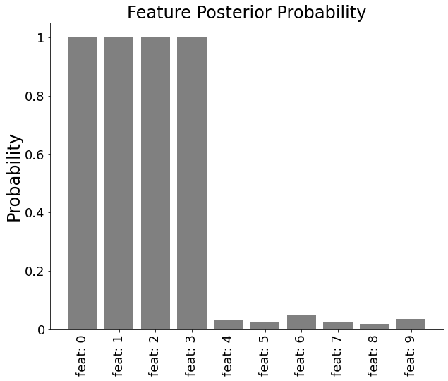
_images/linear_regression_feature_posterior.png

Probabilities for features with nonzero coefficient are close to 1, which indicate that we can select first four features with high confidence. On the other hand, probabilities for dummy features are close to 0.

Sigma posterior distribution

To confirm that defined range of prior distributions properly contains a peak of posterior distribution, plot the posterior distribution of hyperparameters \(\sigma_{\text{noise}}\) and \(\sigma_{\text{coef}}\).

fig, ax = sigma_posterior(
    model=reg,
    title="Log Posterior over ($\sigma_{w}$, $\sigma_{\epsilon}$)",
    xlabel="$\sigma_{w}$",
    ylabel="$\sigma_{\epsilon}$",
    cbarlabel="Log Likelihood",
)

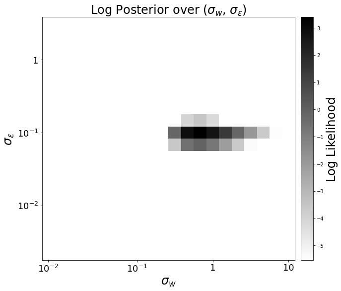
_images/linear_regression_sigma_posterior.png

Peak of the distribution is near the \((\sigma_{\text{noise}}, \sigma_{\text{coef}}) = (0.1, 0.8)\), which is close to the predefined values.

Coefficients

Coefficient values estimated by BMA is stored in ExhaustiveLinearRegression.coef_ attribute.

for i, c in enumerate(reg.coef_):
    print(f"Coefficient of feature {i}: {c:.4f}")

Output

Coefficient of feature 0: 1.0072
Coefficient of feature 1: 0.9766
Coefficient of feature 2: -0.7500
Coefficient of feature 3: 0.5116
Coefficient of feature 4: -0.0006
Coefficient of feature 5: -0.0002
Coefficient of feature 6: 0.0012
Coefficient of feature 7: 0.0003
Coefficient of feature 8: -0.0000
Coefficient of feature 9: 0.0007

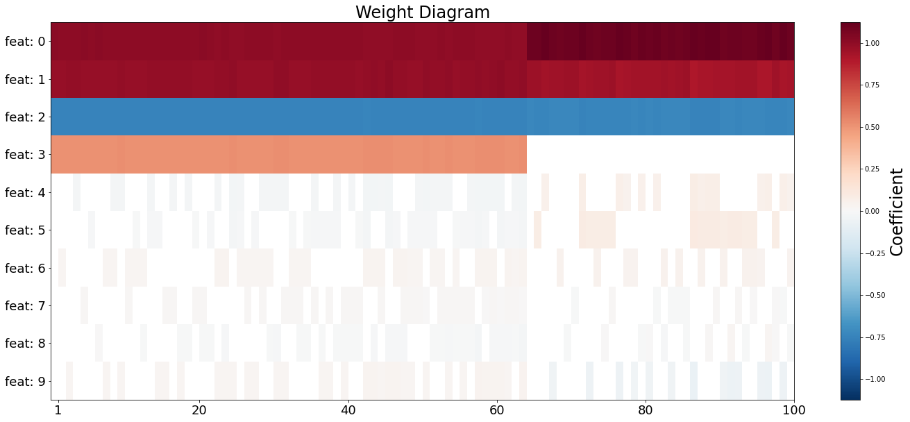
Weight Diagram

For more insights into the model, weight diagram [1] is a useful visualization method.

Prediction for new data

For new data, prediction method is prepared. First, we prepare test data to evaluate the prediction performance.

n_test = 10 ** 3
np.random.seed(10)
test_X = np.random.randn(n_test, n_features)
test_y = np.dot(test_X, w) + sigma_noise * np.random.randn(n_test)

For prediction, we use predict method. Note that data transformation is necessary for feature data and predicted data.

pred_y = y_scaler.restore(
    reg.predict(x_scaler.transform(test_X), mode="full")
)

For performance evaluation, we calculate root mean squared error (RMSE).

rmse = np.power(test_y - pred_y, 2).mean() ** 0.5
print(f"RMSE for test data: {rmse:.4f}")

Output

RMSE for test data: 0.1029

RMSE value is close to the predefined noise magnitude, so the estimation is successfully performed.

References